First of all, let's look at what is Machine learning? ML is simply converting physical representations/data into numbers and finding patterns in them. Deep learning is a subset of ML. In this article, I'll use ML and Deep learning interchangeably. To find patterns in the numbers computers use algorithms that are based on probabilistic methods. In conventional programming, we feed the computer with a set of inputs and rules to follow to get the desired output. But in ML we feed the set of inputs and desired outputs to generate the rules. These rules are figured out by an algorithm and used to deal with the unseen inputs to generate intended outputs which are used to generate the rule in the first place.
If you can build a simple rule-based system that doesn't required machine learning, do that
- first rule of Google's Machine Learning Handbook
It is advisable not to overuse Machine Learning when a rule-based system can fulfil the same functionality. So when to use Deep learning or ML.
When the traditional approaches fails with long list of rules.
For continually changing environments such as autonoumous vehicles.
Discover insights / patterns within large collections of data - such as skin disease classification based on images
When not to use deep learning.
When Explainability of results required. This is due to the uninterpritable nature of the patterns/rules learned by the deep learning models.
When a rule based system is sufficient for the purpose.
When the errors are tollerant.
When the amount of data available is not suffienct even to perform transfer learning.
Deep learning mainly differs from Machine Learning due to the data types which are used to train the models. Typically ML models perform well with structured data whereas Deep learning models perform well with unstructured data. The ML algorithms which are used to create ML models are typically known as "shallow algorithms". Some common examples for ML algorithms are Random Forest, Naive bayers, Nearest neighbour, Support vector machines and etc. Neural networks, Fully connected neural networks, Convolutional Neural Networks, Recurrent Neural Networks and Transformers are the algorithms used in deep learning to create models with unstructured data.
In neural networks, perceptrons are analogous to neurons.
Before feeding data into the neural network the data must be converted to numerical values. This process is called encoding. Then the converted numerical values are fed into a neural network. By using those numerical values the neural network learns feature representations of the data by adjusting the weights and thereby manipulating the gradient values. These feature representation values are used to classify or predict newly inputs fed to the trained neural network. The anatomy of the neural network consists of mainly three components they are namely the Input layer, the Hidden Layer and the Output layer. The hidden layers are used to learn the patterns/embeddings/weights/feature representations/feature vectors all of which refers to the same thing.
The learning process can have three types and are namely Supervised-learning, Semi-supervised, Unsupervised-learning and Transfer learning. In supervised learning, the data and the labels are fed into the algorithm in the training phase. In semi-supervised learning data and some of its' labels are fed into the algorithm in the model training phase. In unsupervised learning, the algorithm learns the patterns by itself only using the input data without the aid of labels. In transfer learning, a pre-trained model is used to learn the representations of data by tweaking the weights.
The practical use cases of deep learning are Recommendation systems, Language translation, Speech recognition, Computer vision and Natural Language Processing (NLP). The deep learning models of the above use cases can be constructed using a library like Tensorflow, Pytorch etc.
The tensors of the neural network are the numerical representations of the input data and the feature representation. A clear intuition about a tensor can be taken from the following video by Dan Fleisch.
With tensor flow, we can simply create a tensor using the following command.
Let's create a tensor with zero dimensions i.e a scaler
scalar = tf.constant(11)
Then check the dimension of the scaler (think about a point)
scalar.ndim
Create a vector
vector = tf.constant([11,11])
Check the dimensions (think about a line)
vector.ndims
Create a matrix
matrix = tf.constant([[11,12,13],
[12,21,11])
Check dimensions (think about a shape)
matrix.ndims
Create a tensor
tensor = tf.constant([ [[11,12,13],
[12,21,11]],
[[11,12,13],
[12,21,11]],
[[11,12,13],
[12,21,11]] ])
Check the dimensions (think about a solid. It could be n-dimensions)
tensor.ndims
The tensors created with the tf.constant are immutable. To allow mutability in a tensor the tensors should be created using the tf.Variable() and then using .assign() the values in the tensor can be changed.
Change the first value of the vector to 12
vector = tf.Variable([11,11])
vector[0].assign(12)
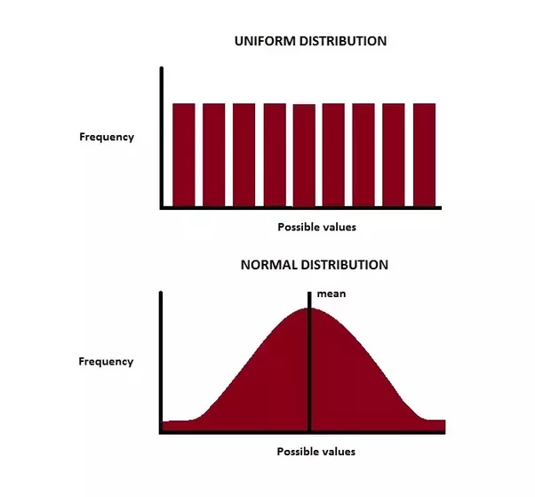
A tensor with random values can be created using a tf.random.normal() or tf.random.uniform() which are used normal distribution and uniform distribution to generate the random values in the tensor respectively.
We can shuffle a tensor using a tf.random.shuffle(<the tensor to be shuffled>). This allows us to shuffle the tensor along its first dimension. By doing so we can avoid the effect of the order of the dataset on the learning of the neural network. For further details read the following.
tf.random.shuffle(
    value, seed=None, name=None
)
Here we can set the operational level seed. To further clarify the use of seed read. Seed is used to get the reproducible experiment results.
We can create tensors with all ones and all zeros as follows.
The NumPy array mainly differs from the tensor is due to the ability of the tensor to run more effectively in the GPU. We can directly convert the NumPy array into a tensor. If required the shape of the tensor also can be manipulated as long as:
A tensor mainly consists of four main attributes. They are namely Shape, Rank, Axis/dimension and Size.
The shape is the length of each dimension of the tensor. Here we could pass the dimension we are willing to get the length.
A.shape
TensorShape([2, 3, 4])
A.shape[0]
2
The rank of a tensor is the number of dimensions a tensor has.
A.ndim
3
The axis or dimension is a particular dimension of a tensor. Here we index the tensor to get the first element of each dimension except for the last one in the first case. In the second case, we get only the first element of the first dimension.
The size is the total number of items in the tensor
tf.size(A)
<tf.Tensor: shape=(), dtype=int32, numpy=24>
tf.size(A).numpy()
24
When dealing with data inferencing using a trained tensorflow neural network almost all the time we may need to change the shape of the tensor. To change and add an extra dimension to the tensor we could use the following.
With TensorFlow, we can perform elementwise tensor division, multiplication, addition and subtraction using tensorflow methods or simply by performing arithmetic operations with your tensor. Matrix multiplication is one of the widely used operations in neural networks and can be performed using tensor. To understand the inner workings of the matrix multiplication click.
Perform matrix multiplication of the tensors (the dot product). The size of the last dimension must be equal to the size of the first dimension of the tensor that is going to be multiplied.
to get the index of the largest value and smallest value we can use
# index largest value
F[tf.argmax(F)]
F[tf.argmin(F)]
Also when you are passing values to a neural network the values should be in numerical form as stated earlier in this article. To convert categorical data to numerical form we often use a one-hot encoding.
# one hot encoding
some_list = [0,1,2,3]# could be red,green,yellow,blue
Infinite division of universe and connection between fractals. The universe is a fascinating and mysterious place, full of wonders and mysteries that we are only beginning to unravel. One of the most intriguing questions that scientists have been trying to answer is whether the universe is infinite or finite and whether it has a simple or complex structure. One way to approach this question is to use the concept of fractals, which are geometric shapes that repeat themselves at different scales, creating patterns that look similar but not identical. Fractals are found in nature, such as in snowflakes, ferns, coastlines, and clouds, but they can also be generated mathematically by applying simple rules repeatedly. Some cosmologists have proposed that the universe itself is a fractal, meaning that it has a self-similar structure at different scales. For example, galaxies are composed of stars, which are composed of planets, which are composed of atoms, which are composed of subatomic part...
There are 5 main steps in training a neural network which is even common for the atomic unit of its perception. Define the network: This could be a lot of layers of neurons. For this case just a perceptron. Prepare the training data: Here we will generate a zero-dimensional tensor with 1000 random values. Define loss and optimizer functions. Optimize use in the training phase to measure and minimize the loss. Train the model with training data to minimize the loss. This is the step we find for what values of weight and bias the training data will fit the model (Here just like y = mx + c ) Validate the model The perception consists of two trainable values namely Weight (W) and Bias (b). As the loss function, we here going to use the Mean squared error loss. 01 Lets define the Perceptron class # Define the model class Perceptron () : def __init__ ( self ) : # initializing the trainable...


Comments